In this guide, we walk through the steps of preparing, uploading, and exploring a circadian dataset using Nitecap.
As an example, the we will use the dataset available here. This contains 24 wildetype (WT) mouse liver RNA-seq samples performed at 4-hour intervals, each with four replicates, under dark-dark conditions, from here. First download the spreadsheet and open it up to examine the format.
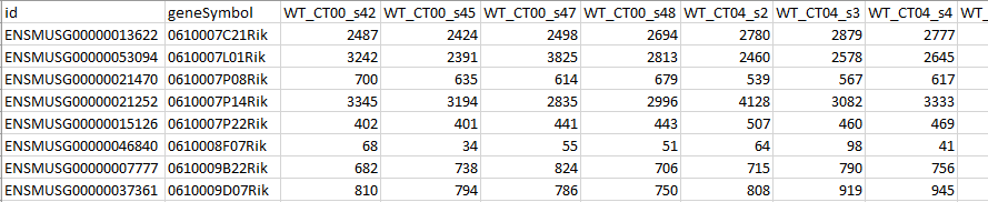
The first row of the spreadsheet gives the column names. Note that the first column has a unique gene identifier (Ensembl gene ID), the second has gene symbols for readable gene identifiers, and the remaining columns are the data for each sample. The sample columns are labelled including "CT00", "CT04", etc.. Unlabelled columns can be used as well, but including labels like "CT00", "ZT00", or "12:00" makes the process easier.
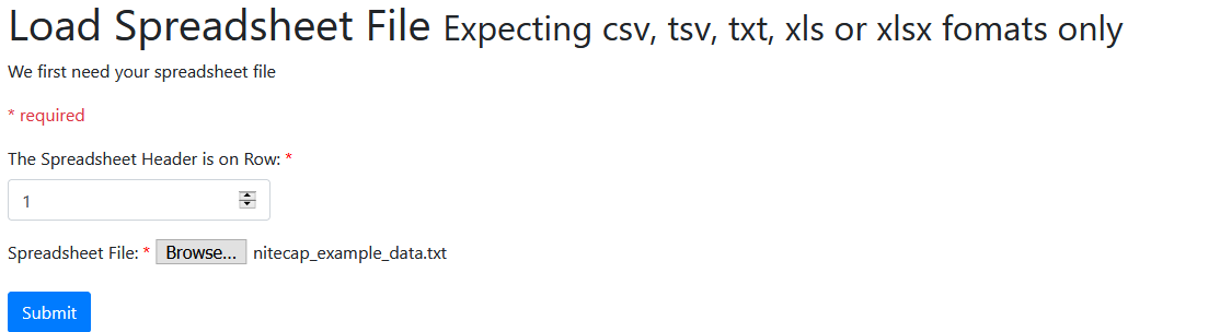
Next, we upload the spreadsheet to Nitecap. From the homepage, click the Load New Spreadsheet button. Since our spreadsheet has the column labels on the first row, we leave the spreadsheet header on row 1. We click browse and select our file to upload. Click Submit and wait for the spreadsheet to upload to our server. Depending on the size of your experiment and internet connection, this may take a little while.
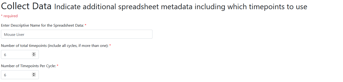
After uploading, we next enter information about our spreadsheet. Choose a good name for the dataset, here we call it "mouse liver". Then enter the number of timepoints in the dataset. This is the number of distinct timepoints that were sampled, not counting multiple replicates of the same timepoint separately. For our spreadsheet, we have timepoints CT00, CT04, CT08, CT12, CT16, and CT20, each with four replicates. Since this is six timepoints we enter six.
Next we enter the number of timepoints per cycle. In our case, we are looking for 24 hour cycles and our dataset just has exactly one cycle. So this has the same value as the previous, and we enter 6 again. Be careful not to accidentally enter one too many here: it's easy to count CT00, CT04, CT08, CT12, CT16, CT20, up to CT24 as one cycle and accidentally enter 7. But the CT24 timepoint is part of the next cycle from the first CT00 timepoint, so we do not include it. As quick check, multiply the number of timepoints by the number of hours between each timepoint - does that equal 24 hours (or whatever period you're investigating)?
Next we need to tell Nitecap what each column means. Nitecap attempts to guess based off of column headers, but if yours don't contain a commonly used label like CT00 or 0:00, then you will have to enter them manually. Each column can be set to "Ignore", "ID", "Stat" or one of the timepoint labels such as "Day 1 Timepoint 1". Choose "Ignore" if you do not want to use the column at all. Choose "ID" for at least one, but possibly more if you want, columns containing feature identifiers. It is always recommended to have unique identifiers, but a second column with more readable names is often convenient, such as gene symbols. Here we select the geneSymbol column as an ID column too so that it will be displayed and the "id" column had been correctly assigned ID already.
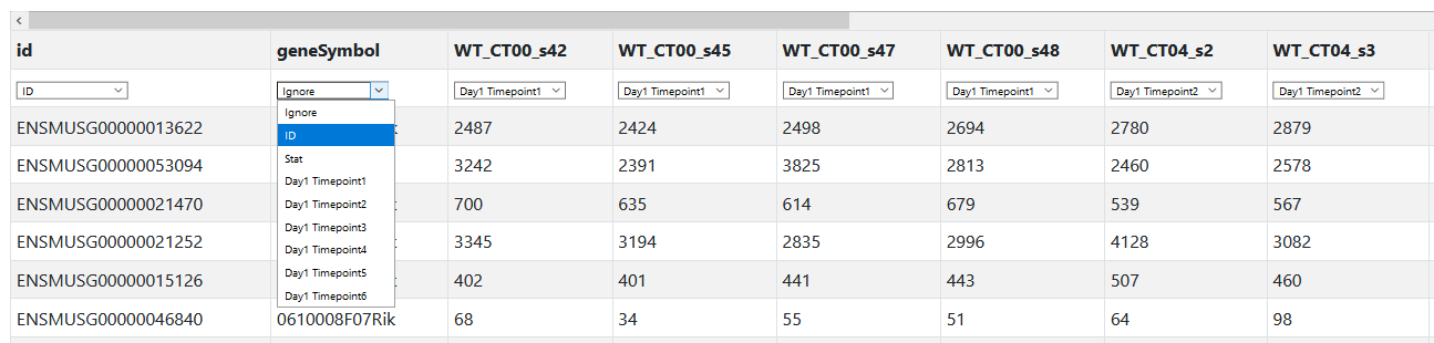
For the other columns, we check that Nitecap has correctly assigned the labels already. For example, CT00 is our first timepoint and the four samples from CT00 are assigned "Day1 Timepoint1". If they had not been, we could set them manually. If we wanted to exclude any of these columns, we could change them to "Ignore".
Finally, note that any additional per-gene level information can be displayed, sorted or filtered by Nitecap alongside the computed results Nitecap provides if you set the column to "Stat". For example, you might include in your spreadsheet a p-value or other statistics computed by an analysis you have already run on your dataset, if Nitecap does not include your preferred statistics already. Or you could include any information about the gene, protein, etc. that you want quick reference to, for example gene biotype. In either case, you could any such columns as "Stat" and find their values alongside Nitecap's automatically generated rhythmic statistics.
After hitting Submit, Nitecap will begin initial processing of your spreadsheet. For large studies, this may take a minute or two. Then you will be redirected to the main spreadsheet viewing page.
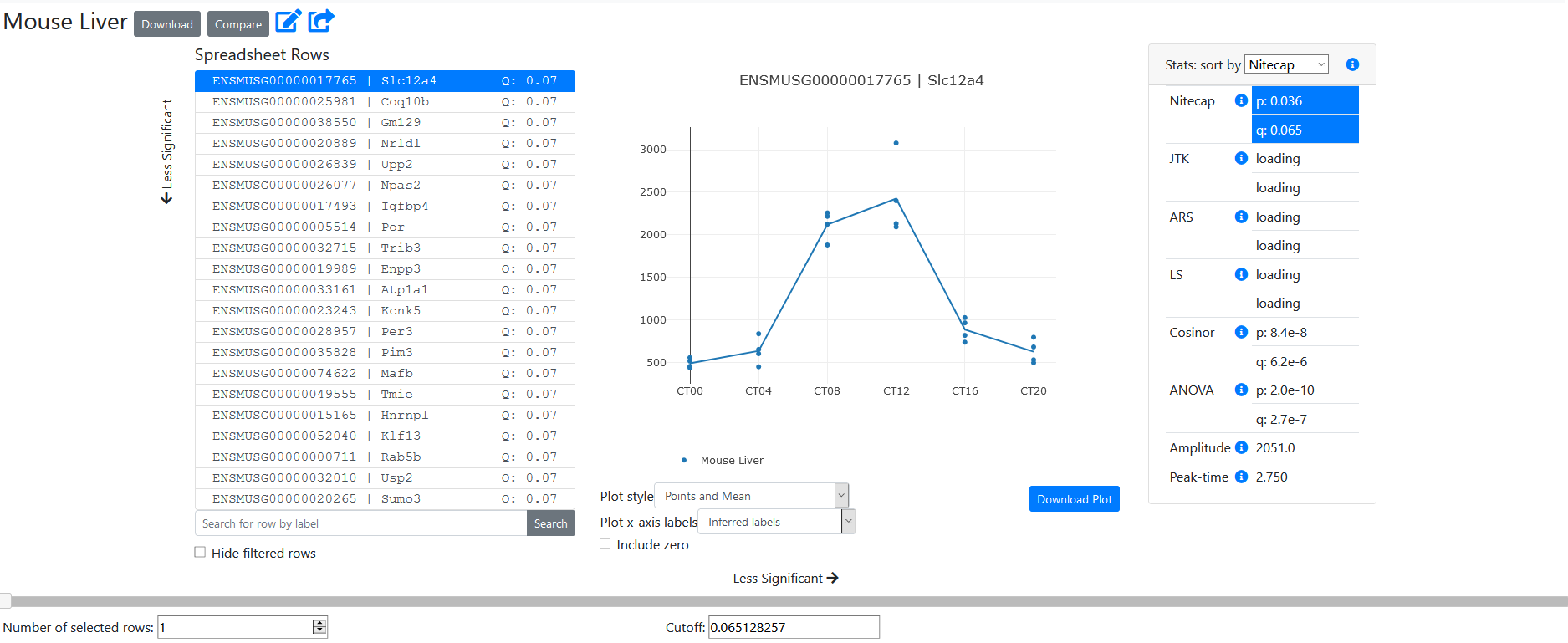
The spreadsheet view page has several features. First, the list of spreadsheet rows shows each feature (here, gene) in the uploaded spreadsheet. The features are sorted according to the chosen statistic from the statistics panel on the right, in ascending order of significance for p-values. The q-value of that statistic is displayed for reference in the row list, if applicable. Since two ID columns were selected, we see the values of both in this list. Note that very long identifiers will be truncated, so we recommend using a small number of ID columns.
Below the row selector, one can search for rows by their identifier. We search for "Arntl", which brings up the gene of that gene symbol, also known as Bmal1, a core clock gene.
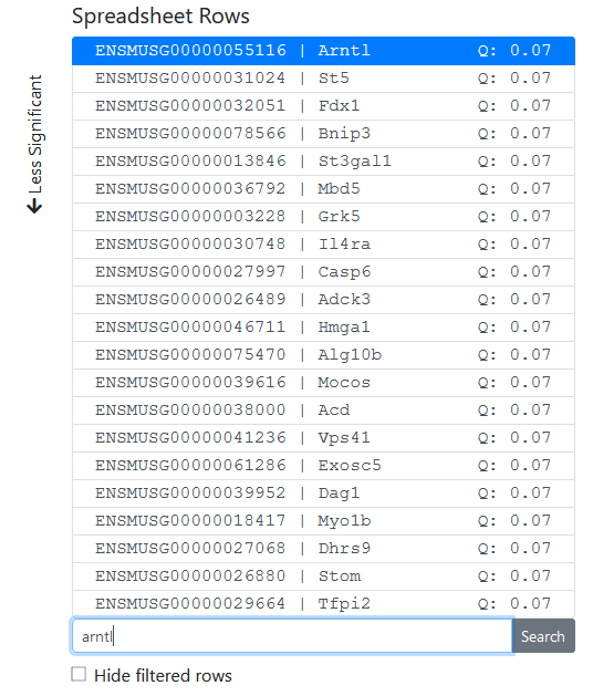
Select "Hide filtered rows" if you have filtered rows out and want them to be hidden from the list (actually, moved to the back of the list) instead of just greyed out. See filtering below.
On the right side, we see the statistics panel. There, we can see the values of all statistics computed from your data. If you provided a 'Stat' column in your data, then it would be displayed here, at the bottom of the list. Otherwise, we see the values computed by Nitecap.
Nitecap will automatically compute for you the following:
You can change the sorting of the rows in the spreadsheet by either click on any of the statistics or by using the drop-down list at the top of the statistics panel.
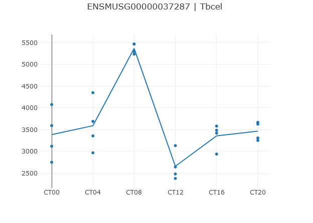
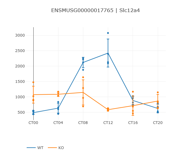
The profile of the selected row is displayed in the center of the page. You can hover over a data point to get its value and sample name.
Below the profile you can select plot style and the x-axis (time) labels. The x-axis labels default to the "inferred labels", which will extract labels from the column headers if the column headers contain "CT00", "ZT00", or "12:00" style labels that are consistent with the metadata. Similarly, "Inferred labels wrapping" will give the same, but will "wrap" back to 0 after 24 hours. You can also select "Include zero" to force the y-axis to always include zero as a baseline.
Press "Download Plot" to download an SVG copy of the plot.
Below the plot is a slider bar, which can be dragged back and forth to "scrub" through the spreadsheet rows. Dragging it to the far left selects the top row, i.e. the most significant one according to the statistic we are ranking by. Dragging it to the far right selects the bottom row, i.e. the least significant. These changes update immediately the profile plot and statistics page. This is useful to examine the overall appearance of a dataset among high, mid or low ranked features.
Use this now to scroll through the dataset and determine approximately where you judge where the approximate transition from rhythmic to non-rhythmic genes occurs in our dataset, after sorting by one of the rhythmicity p-values. This is useful for determining which q-value cutoffs to use for later analysis, to judge the performance of a method, or to check for quality control, such as consistent outliers. Note that our example dataset has a large amount of rhythmicity and you may be able to argue for rhythmicity in a majority of the genes.
Below these, we can set specific cutoffs to go to. First, setting "Number of selected rows" chooses that row number (ignoring filtered out rows, if any). Second, setting "Cutoff" will allow you to set the false discovery rate q-value of the statistic you are sorting for, and to select the top feature below that. Se the cutoff to 0.1, and you will be given the top gene for which the q-value is less than 0.1.
Users of Nitecap should be cautioned against p-hacking
.
Nitecap presents many different methods producing p-values testing rhythmicity or differential rhythmicity and makes re-running downstream analyses quick.
This opens the door to the investigator making choices strategically (or subconciously) to get the desired results regardless of what the data shows.
Investigators should be cautious about using any results that depend highly upon the chosen method or cutoff.
The most reliable results are often those that give similar results under different choices, and investigators should use the multiple analyses methods provided by Nitecap to check for consistency.
Note that since all computed p-values for a specific gene or other feature are computed from the same set of underlying data, they should not be considered as independent.
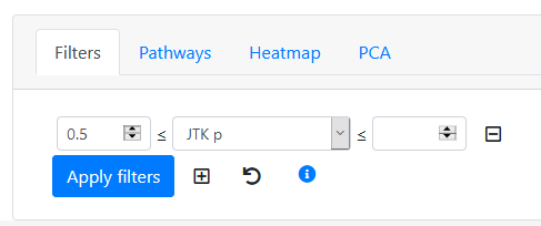
At the bottom of the page are several tabs, the first of which is the Filters tab. Select it now, if it isn't already.
Hit the "plus" button to add a new filter. Select a statistic to sort by from the drop-down list. For example, let's pick "JTK p". Now we can select only genes matching this criteria. Let's examine what non-rhythmic genes look like, so set the left box to 0.5, so that the filter will be choosing only features whose JTK p value is at least 0.5. Then hit "Apply filters".
All rows with JTK p-value less than 0.5 are now greyed out. To move them to the back of the list, we select the "Hide filtered rows" option below the Spreadsheet Row list. Now we scrub the slider bar back and forth to examine the new ordering of genes, with those of JTK p ≥ 0.5 at the front of the list. Choose "ANOVA" and drag the slider bar to the far left. This shows the top ANOVA-ranked gene that is poorly ranked by JTK.
Filters can be removed with the minus sign box to their right. You can also revert to the previously applied set of filters by clicking the circular arrow button.
Delete the JTK p value filter now and hit "Apply filters" so we can continue to see our full dataset.
Nitecap provides basic pathway analysis features for exploratory work. Click the "Pathways" tab. We now must choose a pathway database. Since our dataset is mouse and we have Ensembl gene IDs, we choose one matching that, so we select "Ensembl_Homology_GO_MMusculus". This database is then downloaded.
Next, choose the ID column to sort for pathways on. The first ID column is chose by default, which is correct for our dataset. If you only have one ID column, then this is not necessary to change either.
Hit "Run Pathway Analysis" button and see the results below. We are presented with a list of pathways, ranked according to a hypergeometric enrichment test. The set of genes used is determined according the sorting, filters, and selected row that you have set above. Essentially, any gene passing the filters you've provided and ranked above your selected gene (the one that is displayed in the main profile plot), is considered "selected" and therefore part of the "foreground" set. At the bottom of the results, we can see the number of genes in the foreground list.
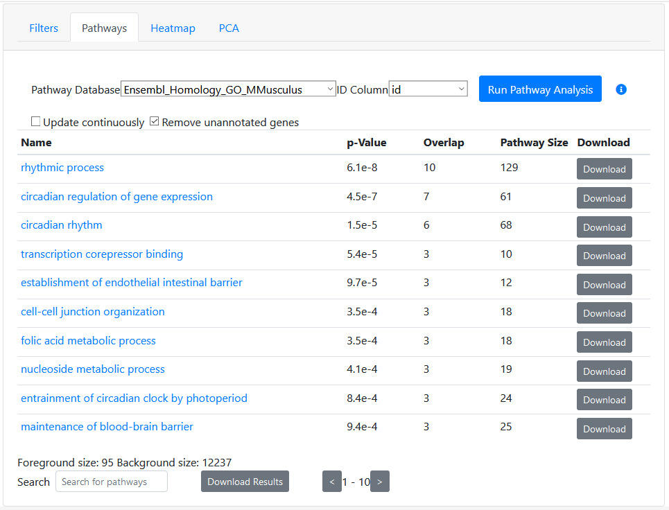
By default, the background list of genes is determined as all genes in the dataset that are annotated in at least one pathway. If you uncheck "Remove unannotated genes" then all genes in your dataset will be considered as part of the background.
To examine how the cutoff changes the pathway analysis, check the "Update continuously" option. Now, any changes to slider bar, chosen sorting, filtering, etc. will be reflected in the pathway analysis in real-time. Scrub through your dataset and see which pathways are enriched at different cutoffs. Check if pathways remain enriched at extremely high cutoffs, which could indicate that the pathways are not well correlated with the feature of interest and instead are enriched due to, say, expression level in that tissue rather than rhythmicity.
We recommend using Nitecap only as a preliminary pathway analysis tool and that all publication-ready pathway analyses be performed in a dedicated tool. The advantage of the Nitecap system is its quick responsiveness and ease-of-use, allowing one to quickly get a feel for a new dataset and how pathway enrichment responds to choice of parameters like the number of genes selected. Using dedicated tools like Ingenuity Pathway Analysis or GSEA will give you better pathway lists for your finalized pathway enrichment analysis.
You can download results of the pathway enrichment to examine them further. For individual pathways, download buttons are on the right of the results table and provide the list of genes in the pathway and the genes overlapping in both pathway and our data set's selected genes. For the entire set of pathway enrichments, you can download the summary in the "Download Results" button at the bottom.
One can also search for a specific pathway by name, or page through the list of results to see past the top 10.
Heatmaps provide quick and easy visualization of the behavior of a moderately large number of genes, but cannot show more than a few hundred genes. Click on the Heatmap tab and the "Generate Heatmap" button.
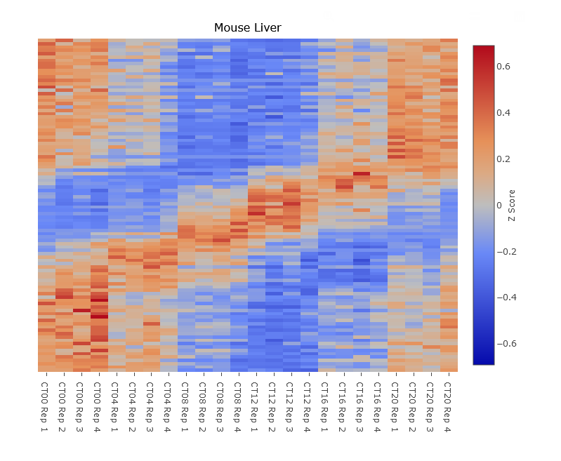
The set of features shown in the heatmap depends upon your selected rows, just as in the pathway analysis. Specifically, it takes all features that rank at least as highly as the selected feature (shown in the main profile plot) that are not filtered out (shown in grey in the row selector list). Therefore you can use the slider bar, set a number of selected features, or set a cutoff value to determine how many features to display in the heatmap. In the example figure, we have set it to sort by JTK and selected the top 100 genes. Note that if you include more genes than there is space to display, only a subset of rows will be displayed until you zoom in.
Each row in the heatmap shows that data of one feature. The data has been z-scored (i.e. that feature's mean and standard deviations have been set to 0 and 1, respectively), so that values are comparable across different scales. White indicates the average value of that feature across all timepoints.
A heatmap takes the set of selected genes are re-sorts them according to their peak time (aka acrophase). This creates a more readable visualization for most datasets since similarly timed genes will be side-by-side. If this were not done, then they would be sorted by significance and nearby genes, while both significanly rhythmic, would likely be entirely out of phase and the plot would be extremely difficult to read. However, in some circumstances (such as small datasets with few timepoints and no replicates), this can create the appearance of patterns that are not likely to be replicable.
You can also adjust the plot combine replicates of the same time points together, to combine multiple cycles of data into one (if you dataset contains multiple cycles), or to show row labels (from the ID columns). Note you should only choose to show row labels if there is a fairly small number of rows, anything more than around 50 is unreadable and may be slow to render.
The PCA plots provide a way to view the bulk rhythmic behavior of a condition. Like heatmaps and pathway analysis, Nitecap performs PCA on the set of features you have selected. Specifically, it takes all features that rank at least as highly as the selected feature (shown in the main profile plot) that are not filtered out (shown in grey in the row selector list). This contrasts with a more standard PCA which would include all features. Users can still generate those by selecting all features (dragging the slider bar to the far right). However, we find that running PCA on different sets of features can be highly informative, and we encourage investigators to try multiple options.
For our example, select the top 500 genes sorted by JTK p-values and hit "Run PCA."
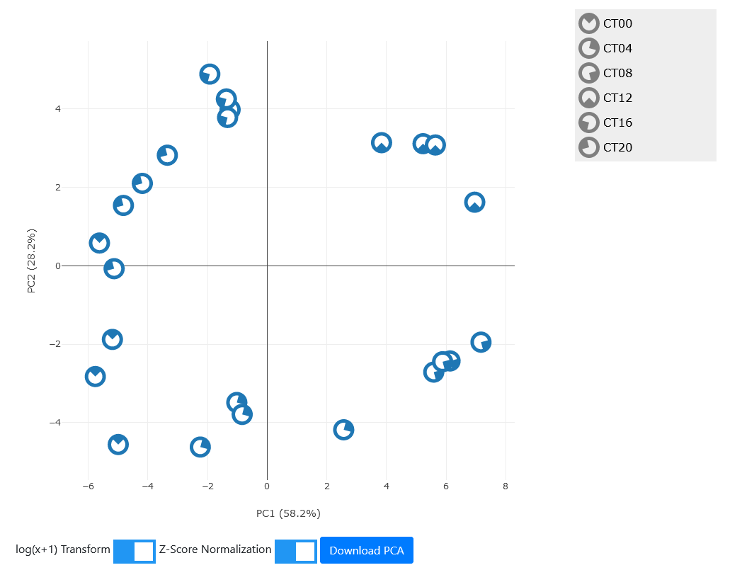
Since this dataset has strong rhythmicity in the selected genes, we observe that the PCA plot forms a circular shape with the samples of the same timepoint clustering together, and timepoints in order around the clock. The PCA displays the timepoint with a "PAC-MAN" shape indicating the time of day. Note that choice of signs in PCA is arbitrary so while sometimes plots like these have the timepoints going clockwise and sometimes have them going counter-clockwise, there direction is completely arbitrary.
PCAs are particularly informative for comparisons of different datasets, for example a wild-type versus a knock-out mouse to explore the effects of the knock-out.
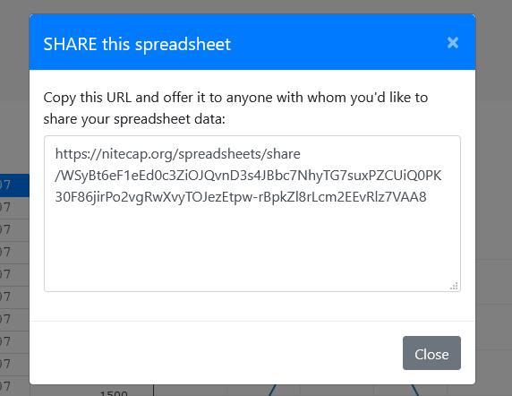
Next to the dataset name, there are several buttons. Press the arrow-shaped "Share" button to create a shareable link to your dataset. Copy-and-paste the provided link and you can give it to any colleague to use to see your dataset, including your chosen sorting, filtering, and selected rows.
You must be logged into an account in order to create these shareable links. Accounts are free and allow your uploaded datasets to be stored for later use.
Nitecap provides support for comparing rhythmicity among different conditions, such as between wildtype and knock-out mice or between a control and treatment group. In order for two datasets to be comparable, you must first upload each of them as described here. Only spreadsheets with the same study design are currently supported for comparing: they must have the same numbers of total timepoints and the same number of timepoints per cycle in their metadata. However, they do not need to have the same number of replicates at each timepoint. Additionally, the spreadsheets need to have matching ID columns, with some IDs common to both datasets. Check that you have chosen the same ID types as ID columns in both spreadsheets and that they both have the same number of ID columns set in the metadata (click the "Edit" button while viewing a spreadsheet to check this).
If two datasets match these requirements, it still may be inadvisable to compare them if they were not produced as part of a single study. For example, comparing two studies from different labs or different years may be possible but not recommended as the differences observed will be technical in nature.
To compare the datasets, there are two easy ways. First, you can click on "Display Spreadsheets" at the top of the page (while logged in) to access the list of your stored spreadsheets. Then, select two spreadsheets and hit the "Compare" button. Alternatively, open one spreadsheet first, then hit the "Compare" button next to the dataset name at top. Then a list of comparable datasets is displayed. Click the name of the spreadsheet you'd like to compare to and that comparison will open.
If you do not have a second dataset, you can experiment with a shared comparison here.
Viewing the comparison gives a similar view as in a single dataset. The rows of the spreadsheets are matched by their ID columns. Any rows without matches in the other spreadsheet are dropped from the comparison. The central profile plot shows the profile of the feature in both conditions, colored accordingly.
Note that Nitecap automatically attempts to generate shortened condition names from your two study names. Parts of the study names that are the same in both datasets will be dropped for simplicity. So it is recommended that you give consistent dataset names such as "Study 1 Control" and "Study 1 Case", which will result in readable labels of "Control" and "Case".
In addition to all the single-dataset statistics (including user-uploaded statistics), Nitecap computes additional comparisons statistics. These are:
You can now choose to sort by statistics from either dataset, or shared statistics from the comparison. Note that sorting by JTK p-values, for example, will be done for one dataset or the other without incorporating the other spreadsheet at all. Make sure to check which spreadsheet the sorting is applied to by checking where the blue highlighted statistic is in the statistics panel. To change which spreadsheet it is sorting by, just click the statistic under the corresponding header in the statistics box.
All the advanced analysis tabs (filters, pathways, heatmap, and PCA) at the bottom work as well on comparisons. In particular the PCA plots are highly useful. For our example, select a set of rhythmic genes in the wild-type mice. For our example here, select 350 top rhythmic genes in the WT (wild-type) condition and generate the PCA.
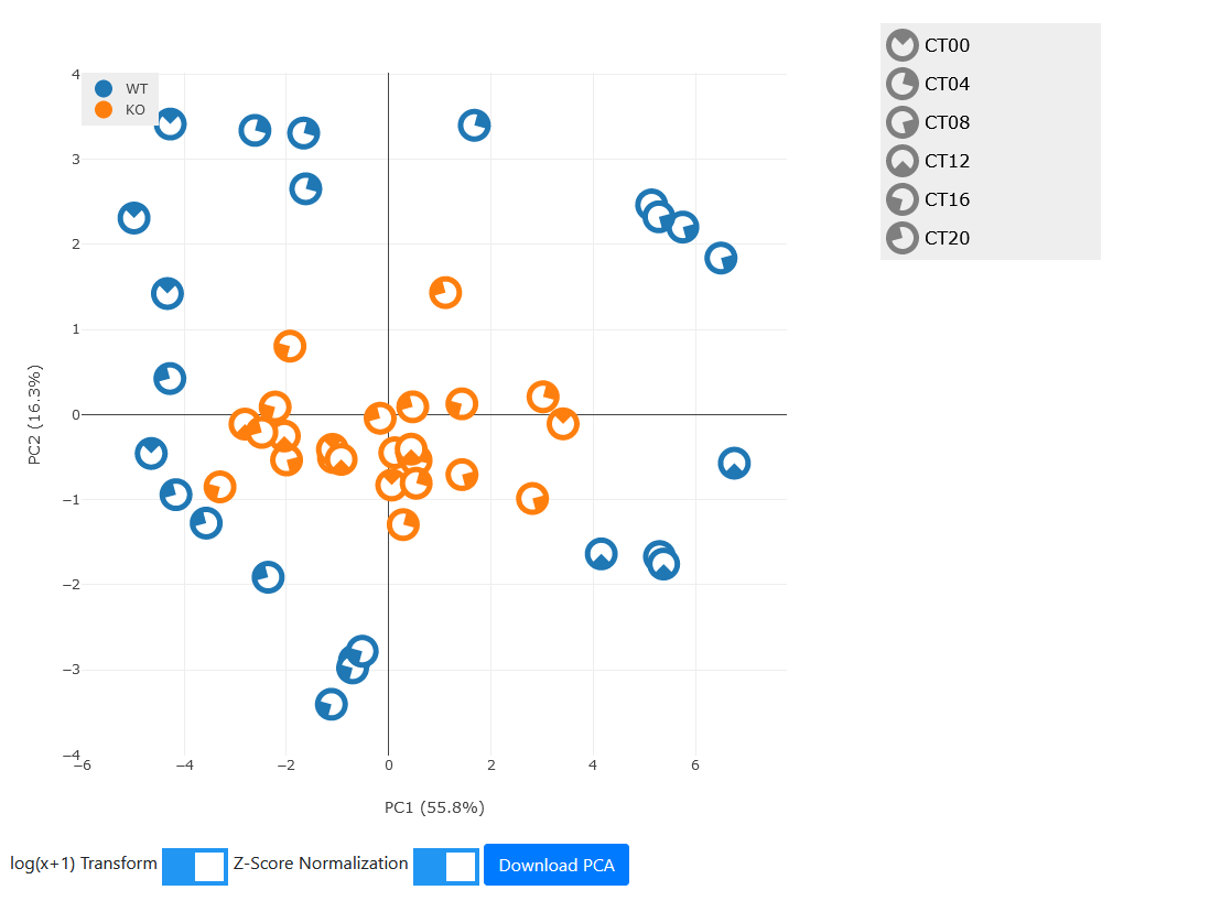
Observe that the rhythmicity of the wild-types is evident from the clustering by timepoints along a circular arc. However, in the knock-outs we can clearly see that the dataset has greatly reduced rhythm in the selected genes and indeed does not separate by timepoint at all.